1.
Introduction
blueSeed Plan is a productivity desk application developed to help users
building up a Business Plan, specifically, within the main areas of this
process, would assists the user in foreseeing budgets and projections to show
financial outcomes of an already ongoing project or one under discussion. An
essential tool for entrepreneurs or businessmen, taking their first steps in a
new undertaking or start-up, to evaluate its viability. It is very helpful when
carrying out financial, economic or costs analysis, above all in the case you
need to address potential investors interested in your project in funding
rounds, for example.
Taking into account common
data from the accounting records in the administration software or ledgers of
the company (sales, staff costs, inventory, financial expenses and revenues,
etc.), this app will lead you through the process of making up your own
financial forecasts in a very easy way. You will be able to produce some
projected statements as: Income Statements, Balance Sheets, Cash Flow
Statements, Break Even Analysis and Sources and Uses of Funds.
Besides the
accounting information, blueSeed Plan would ask you to introduce some global economic
variables such as CPI and Market Interest Rate. Depending on the exactitude of this
values and enterprise operational ones (you will find different sections, in
the user interface, where you will be asked to fill diverse kind of data a
company works with), you would have more accurate figures.
The reports issued by
this app would describe in numbers the outcome of your business strategies and
policies. They would help to provide an operating plan to assist you in running
the business and improve your probability of success.
The application is
divided in various sections:
2.
Global Variables
The first time you
run the application or when you select to create a new document (or Project as it is called by the program),
you would be asked to introduce the Global Variables for the current document
which are: number and kind of periods, currency, CPI and Interest Rate of your
country or geographical area.
They will be used to
calculate price variation through the inflation rate, financial expenses and
revenues, and compound interest for all products in the company portfolio.
Hereunder, you can
see a screenshot of the first form and dialog boxes where you should insert the
figures:
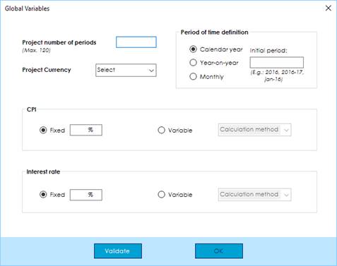
You should introduce
data in the following fields:
3. Project Number Of Periods
Within this part you
should write the number of periods (years or months) your project will have, with
a maximum of 120. You should put an integer in the textbox without comas or any
other character.
This number would be
the time horizon you will set for all projections and must fit our and the
target audience expectations for this exercise.
4. Period Of Time Definition
As you can see in the
previous image there are three format options for each time unit (either year
or month) of the project:
·
Calendar year: periods of time
started in January and ended in December (natural year), you should put the
four digits of the initial year, for example:
“2016”, “1981”.
·
Year-on-year: this biannual format
can be used for not natural years, would be the case of fiscal or economic
years starting in a different month than January and not ending in December, the
way to write them is putting the four digits of the first year, hyphen followed
by the last two digits of the second year, for example: “2016-17”, “1981-82”.
·
Monthly: you can use this
format if you want to set a period of time lesser than a year, then select a
starting month and have in mind this time subdivision would be maintained
through all the time horizon. You should write the first three letters of the
starting month, then a hyphen followed by the last two digits of the initial
year, for example: “ene-16”, “jun-16”.
When you choose this
option, the application will automatically add a column with aggregated figures
in some of the reports produced, such as Income Statement, Balance Sheet, etc.
If you leave blank
this textbox the program will name “Period” to all time units and will number
them consecutively.
5. Currency
Although it has no
impact in any calculation made by the application, you can choose a name or a
symbol for the currency of the project, either one of which appear within the dropdown
box in the related subject or clicking “Other” in the same dropdown box and
writing the desired name in the appearing textbox.
The selection will
appear in all the reports produced.
You can also leave it
blank, in that case there will be no reference to any currency in the issued
reports.
6. CPI
CPI (or Consumer
Price Index) is a variable that would affect to several items in the project, such
as products sales prices, wages, purchasing and overheads, just like what
inflation reflects when price indexes increases.
For our project, it
can be a signed or unsigned integer or floating with two decimals at best.
Furthermore, this rate can be fixed for all the project, meaning that price
variation will be the same for all periods, or variable, you can put a
different rate for each period.
If you want a fixed
CPI you should put the desired estimated figure in the textbox labeled for that
purpose, on the other hand, if you want a variable rate the program gives you
four alternatives for its calculation:
1.
Manual
When you click on
this dropdown box item, a new form will appear with a blank table where you can
manually insert CPI figures for each period. They can be signed or unsigned
integers or floating numbers with decimals.
2.
Linear
Coefficient
When you choose this option, the form shows a textbox
where you can put the CPI rate for the first period (rate expressed in
percentage), and then the increase or decrease to apply in all other periods (in
this case this rate should be expressed in per-one, e.g. for a 10% rate change
you should write “0.01”).
The application will calculate future rates for each
period of time applying that linear coefficient each time over the previous.
3.
Data
Import
blueSeed Plan allows data import from an Excel file. So once you
have chosen that option in the dropdown box and an Excel file in the subsequent
window, you will see a similar form to the previous ones:
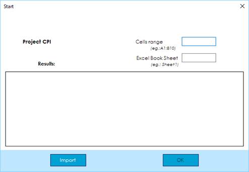
First of all, you should put the cells range containing
the data to import in the textbox labeled that way (data can only be numbers,
this option does not accept text), and it can have several rows and columns. If
the range has more than one row, the application takes values from left to
right and top to bottom.
Next step is to write the name of the Excel worksheet
in the next textbox under the previous one.
Then you click on “Import” and wait until the blank
table is filled with the numbers in the Excel file (this process could take
long if the selected range is too big).
If everything has worked out correctly and the figures
in the table are the ones you wanted, you can click on “OK”, otherwise you can
repeat the process checking the range and name of the Excel worksheet.
4.
Time
Series
Last item in
the dropdown box is “Time Series”. blueSeed Plan provides another
calculation method to estimate CPI rates in the Project. It do it according to historic
data trends, adding every new obtained value to the calculation of the next
period of time rate.
Once you have
the Excel file, where you keep the data series, selected (cells values can only be numbers, this
option do not accept text) you will see a similar form to the previous one. Here
you will first have to put the cells range in the upper textbox, it can have
several rows and columns, if it has more than one row, the application takes
values from left to right and top to bottom. Then you write the name of the
Excel sheet in the bottom textbox.
You click on “Import and calculate” and wait until the
blank table is filled with the numbers calculated by the application (this
process could take long if the selected range is too big).
If everything has worked out correctly and the figures
in the table seem to be right, you can click on “OK”, otherwise you can repeat
the process checking the range and name of the Excel worksheet.
7. Interest Rate
Interest Rate is a
global variable (it would be the reference value for all the interest rates
needed in the project) and would affect to several items in the project, such
as leasing, renting, loans or credit lines. It can be a signed or unsigned
integer or floating with two decimals at best.
Besides, this rate
can be fixed for all the project, meaning that price variation will be the same
for all periods, or variable, you can put a different rate for each period.
If you want a fixed Interest
Rate you should put the desired estimated figure in the textbox labeled for
that purpose, on the other hand, if you want a variable rate the program gives
you four alternatives for its calculation:
1.
Manual
When you click on
this dropdown box item, a new form will appear with a blank table where you can
manually insert Interest Rate figures for each period. They can be signed or
unsigned integers or floating numbers with decimals.
2.
Linear
Coefficient
When you choose this option, the form shows a textbox
where you can put the Interest Rate for the first period (rate expressed in
percentage), and then the increase or decrease to apply in all other periods (in
this case this rate should be expressed in per-one, e.g. for a 10% rate change
you should write “0.01”).
The application will calculate future rates for each
period of time applying that linear coefficient each time over the previous.
3.
Data
Import
blueSeed Plan allows data import from an Excel file. So once you
have chosen that option in the dropdown box and an Excel file in the subsequent
window, you will see a similar form to the previous ones:
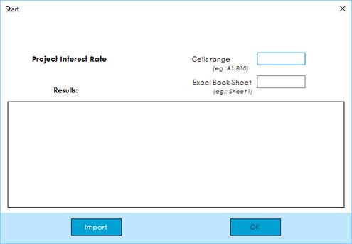
First of all, you should put the cells range
containing the data to import in the textbox labeled that way (data can only be
numbers, this option does not accept text), and it can have several rows and
columns. If the range has more than one row, the application takes values from
left to right and top to bottom.
Next step is to write the name of the Excel worksheet
in the next textbox under the previous one.
Then you click on “Import” and wait until the blank
table is filled with the numbers in the Excel file (this process could take
long if the selected range is too big).
If everything has worked out correctly and the figures
in the table are the ones you wanted, you can click on “OK”, otherwise you can
repeat the process checking the range and name of the Excel worksheet.
4.
Time
Series
Last item in
the dropdown box is “Time Series”. blueSeed Plan provides another
calculation method to estimate CPI rates in the Project. It do it according to
historic data trends, adding every new obtained value to the calculation of the
next period of time rate.
Once you have
the Excel file, where you keep the data series, selected (cells values can only be numbers, this
option do not accept text) you will see a similar form to the previous one.
Here you will first have to put the cells range in the upper textbox, it can
have several rows and columns, if it has more than one row, the application
takes values from left to right and top to bottom. Then you write the name of
the Excel sheet in the bottom textbox.
You click on “Import and calculate” and wait until the
blank table is filled with the numbers calculated by the application (this
process could take long if the selected range is too big).
If everything has worked out correctly and the figures
in the table seem to be right, you can click on “OK”, otherwise you can repeat
the process checking the range and name of the Excel worksheet.
8. Project Start
Once you have all global variables well defined within
the first form, you should validate clicking on the corresponding button. If
there is no errors, “Accept” button is activated so it can be clicked to
continue with following stage in the process.
Now you have press the button, current window disappears
and the main window of the program is showed. Here you will introduce specific
data of the project.
You can see a detail of this form hereunder:
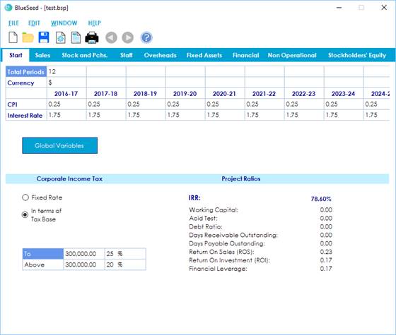
As you can realize this form has several tabs in it. The
one selected is the one is opened in first instance every time you start a new
project (“Start”).
First thing you can appreciate in the upper part is a
table with a summary with the numbers you have already introduced in the first
window. This table cannot be modified without going back to the first form, and
for that you would have to click on the “Global Variables” button below.
In the case you could not see all the columns or rows
of this table, you can click on it and move through the cells with the arrow
buttons in your keyboard.
If you are compelled to change any of those first
variables, you should bear in mind that depending on what changes are you going
to do, they may affect to the information you have already put in the main
window (in any of its tabs) and in some cases lose some part of it.
In the lower part of the tab you can see two captions:
Corporate Income Tax, which we explain in the next section, and Project Ratios where
you can find a list of several financial rates you can use for your analysis. This
ratios are refreshed every time we ask for a report in the application menu or
tool bar.
Corporate
Income Tax
In this block you can define sort of and rates for the
Corporate Income Tax. If it is a fixed rate type or it is a tax bracket one,
then select bracket ranges and income tax rate for each one.
For fixed rates, you just have to write the desired
figure in the textbox of the window that will appear when we get in “Fixed Rate”
box, then you click on “OK” and the number will be displayed in the textbox. It should be an unsigned integer or
floating with two decimals at best.
For tax bracket type, first step is to select the radio
button labeled as “In terms of Tax Base” and a dropdown box and two more
textboxes will be displayed. To define the tax bracket structure you may
proceed as follows:
-
The dropdown box lists two items: “To” and “Above”. Every time you want
to set a new bracket you have to select “To” except in the case of the last
bracket, where you have to clink on “Above”, thus adding last row of the table
and closing the bracket structure.
For instance, for a tax structure of three brackets: 0-100,000,
100,001-300.000 and 300,001- ∞, you would have to
put “To” in the first two segments, and “Above” in the last one.
-
In the textbox under the dropdown box, you have to write the figure corresponding
to the upper limit of the Tax Base (net income before taxes) Bracket, except for the last one where
you leave the previous number as the lower limit in a bracket that has no upper
end (or it has ∞).
Following prior example: 100,000 for the first one,
300,000 for the second one, and you will leave 300,000 for the last one.
-
Finally, you can insert tax rate
for every bracket in the second textbox, it should be an unsigned integer or
floating with two decimals at best.
For example, in a tax
structure which seeks to benefit low profits: 20% for the first bracket, 25%
for the second and 30% for the last one).
Once you have the values you require in the
corresponding boxes, you click on “Add to list” every time you want to
introduce a new bracket in the table. Any time you do it for the last segment
of that range (when you have “Above” selected in the dropdown box), you will
see this button and the one named “Delete row” will disable, as you have
already completed the tax income bracket structure.
To revert that situation you have to click on “Fixed
Rate” radio button and the table and boxes will disappear.
Before having introduced the last bracket in the table,
when it is not blocked and accepting more fields, you can delete rows of that
table by just selecting the one you want to delete and clicking on “Delete row”.
Now you have to
continue introducing data in the next tabs, so we will go over each one of the
in the following sections.
9. Sales
Sales tab shows the
following view:
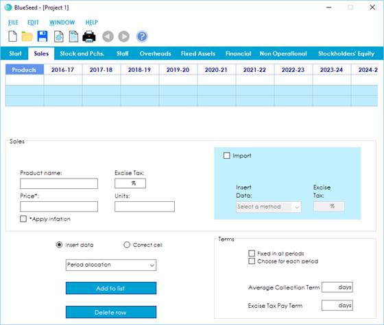
First thing you see
is a blank table (with the exception of the headers on every column) where you
will see displayed every data you will be introducing afterwards: name of the
products (in the first column), sales amounts by period of time (next columns
with the periods names in the header), collection and excise tax pay terms by
period of time (which will be shown in the last two blue rows) and, finally, excise
tax rate by product (in the last column of the table, which cannot be viewed in
upper image).
In the case you could not see all the columns or rows
of this table, you can click on it and move through the cells with the arrow
buttons in your keydoard.
There are two ways to
insert data in the table: manually one by one or importing values from an Excel
worksheet.
In the first case you
should fill the different dialog boxes: product name, price (not excise tax
affected), excise tax rate and number of units sold. Then you should allocate a
period of time in the dropdown box just over the “Add to list” button.
If you want product price
to be affected by CPI (the value you have introduced in the first form), we
tick on the checkbox labeled “Apply inflation”. The way in which the program take
into account the inflation rate is to apply a coefficient to the price you have
written in corresponding textbox (which should be a reference from the previous
period to the first one in the project). That coefficient is the result of
multiply all the CPI rates (the ones shown in the table in the firs tab) from
the first period of time to the period you have currently selected.
Now that you have all
the data you want to introduce in the table and the period of time where you
want to do it, you can insert that values by clicking on “Add to list” button.
Average collection
and Excise Tax pay terms are added separately selecting one of the two options
in the “Terms” section, fixed for all the project, with means they would be the
same terms in all the periods of time, or you can select to put different terms
period by period (in this case you will see that the dropdown box used to
allocate periods is enabled).
To correct any of the
figures you have already introduced in the table, you count with two options: you
can delete a complete row (or product) just by selecting it and clicking on “Delete
row” button, or you can correct individual values cell by cell.
To change values in
only one cell you first have to select the radio button labeled as “Correct
cell”, then you have to select the cell by clicking on it and press “Correct”
button. A new window will appear where you have to introduce a new value, click
“OK” and the cell will show amended figure.
Import
As explained before, the application allows data
import from an Excel worksheet, as an alternative to inserting numbers one by
one as described in the manual method above.
To start this option you have to check “Import” box, write
excise tax rate if applicable within the textbox enabled, and then select one
of the two methods the dropdown box offers to the users:
1)
Data Import
First option is plain data import, once you have
chosen the Excel file where you have the information you want to import, in the
dialog window appearing after clicking on the corresponding dropdown box item,
you will see a similar form to the previous ones (CPI and Interest rate import
methods), and also process to follow is quite similar.
First of all, you should put the cells range
containing the data to import in the textbox labeled that way, but here there
is a difference this time in the way the values has to be positioned. They
should be organized in a similar way the application ask for values when using
the manual method, so there are two key factors to have in mind before organize
the information in the Excel worksheet:
I.
First column of the range should
contain the name of the products (with as many rows or fields as you need).
II.
After this first column, they
should follow pairs of columns for each same period of time (product price and
units sold, and should be as many pairs of columns as periods of time in the
project), with the same number of rows than the first one.
Next step is to write the name of the Excel worksheet
in the next textbox under the previous one.
Then you click on “Import” and wait until the blank table
is filled with the names and numbers in the Excel file (this process could take
long if the selected range is too big).
If everything has worked out correctly and the values
in the table are the ones you wanted, you can click on “OK”, otherwise you can
repeat the process checking the range and name of the Excel worksheet.
2) Time Series
The second item
listed in the “Insert data” dropdown box within import section is “Time
Series”. blueSeed Plan provides another
calculation method to estimate total sales figures for each period of time (for
only one field or product each time). It do it according to historic data
trends (data provided by the user), adding every new obtained value to the original
series and using increased set of values for the calculation of the next period
of time rate.
Once you have
the Excel file, where you keep the data series, selected (cells values can only be numbers, this
option do not accept text) you will see a similar form to the previous one.
Here you will first have to put the cells range in the upper textbox, it can
have several rows and columns, if it has more than one row, the application
takes values from left to right and top to bottom.
Then you write the name of the Excel sheet in the bottom
textbox.
It is important to note that, firstly, the program asks
only for historic sales figures (not prices at all, and not units numbers yet),
and no need neither to introduce names of the products in the first column as
before (application will assign a default name).
You click on “Import and calculate” and wait until the
blank table is filled with the numbers calculated by the application (this
process could take long if the selected range is too big).
When the program has finished calculation of the total
amount of sales for each period of time, it announce the user he could now
introduce total units sold in for each period, another table appears where we
can introduce, manually this time, the total quantity numbers for each period
(this table can be left totally blank as it has not impact in sales now that
the first table is completed).
If everything has worked out correctly and the figures
in both tables seem to be right, you can click on “OK”, otherwise you can
repeat the process checking the range and name of the Excel worksheet.
10. Stock And Purchasing
Stock and Purchasing tab has the following appearance:
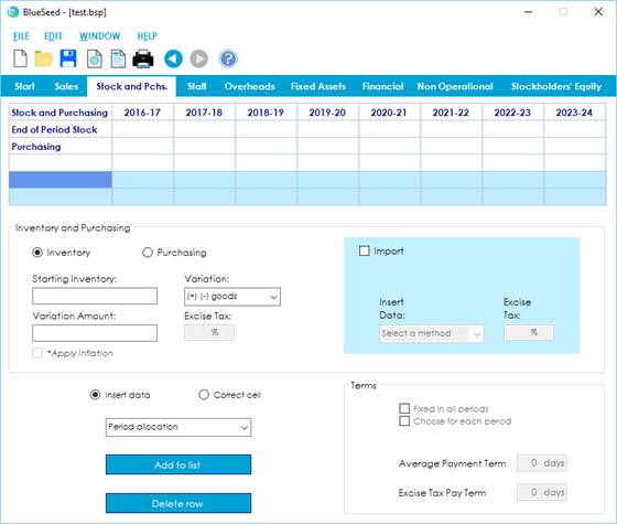
Just like in the previous
tab, first thing you see is a blank table (with the exception of the headers on
every column and two first rows). Here you will see displayed every data you
will be introducing afterwards: end of period goods stock figures (in the first
row), name of the purchased products (in the first column under “Purchasing”
header), purchasing amounts by period of time (next columns with the periods
names in the header), average and excise tax pay terms by period of time (which
will be shown in the last two blue rows) and, finally, excise tax rate by
product (in the last column of the table, which cannot be viewed in upper image).
In the case you could not see all the columns or rows
of this table, you can click on it and move through the cells with the arrow
buttons in your keyboard.
To select the kind of
data you are working with, inventory or purchasing, you first have to click on
the consistent radio button, and follow as described in next paragraphs.
There are two ways to
insert data in the table: manually one by one or importing values from an Excel
worksheet.
In the first case you
should fill the different dialog boxes. When you are inserting inventory
figures you find a first textbox where you have to put opening balance in, beside
there is a dropdown box where you should specify during the period the goods
stock has increased or decreased, finally, in the textbox below you write the
amount of stock variation. Then you allocate the period of time to which the
data is related in the dropdown box just over the “Add to list” button.
Otherwise, if you are
introducing purchasing information, you first have to write the name of the
good in the upper textbox, then the purchased amount for that period, an excise
tax rate if applicable. Then again, you allocate the period of time to which
the data is related in the dropdown box just over the “Add to list” button.
If you want purchased
goods price to be affected by CPI (the value you have introduced in the first
form), we tick on the checkbox labeled “Apply inflation”. The way in which the
program take into account the inflation rate is to apply a coefficient to the purchased
total value you have written in corresponding textbox (which should be a
reference from the previous period to the first one in the project). That
coefficient is the result of multiply all the CPI rates (the ones shown in the
table in the firs tab) from the first period of time to the period you have
currently selected.
Now that you have all
the data you want to introduce in the table and the period of time where you
want to do it, you can insert that values by clicking on “Add to list” button.
Average and Excise Tax
pay terms are added separately selecting one of the two options in the “Terms”
section, fixed for all the project, with means they would be the same terms in
all the periods of time, or you can select to put different terms period by
period (in this case you will see that the dropdown box used to allocate
periods is enabled).
To correct any of the
figures you have already introduced in the table, you count with two options: you
can delete a complete row (or product) just by selecting it and clicking on “Delete
row” button, or you can correct individual values cell by cell.
To change values in
only one cell you first have to select the radio button labeled as “Correct
cell”, then you have to select the cell by clicking on it and press “Correct”
button. A new window will appear where you have to introduce a new value, click
“OK” and the cell will show amended figure.
Import
As explained before, the application allows data
import from an Excel worksheet, as an alternative to inserting numbers one by
one as described in the manual method above.
To start this option you have to check “Import” box,
write excise tax rate (just in the case you are working with in purchasing
choice) if applicable within the textbox enabled, and then select one of the two
methods the dropdown box offers to the users:
1)
Data Import
Subject to what kind of values you have chosen to
introduce, inventory or purchasing, the way the information has to be ordered
in the worksheet is going to vary, so we now are going to show you the two
different cases:
a)
Inventory
Once you have selected the Excel file in the window
appearing after clicking in the dropdown box item, you must follow next
instructions:
First of all, you should put the cells range
containing the data to import in the textbox labeled that way (data can only be
numbers, this option does not accept text), and it can have several rows and
columns. If the range has more than one row, the application takes values from
left to right and top to bottom.
Next step is to write the name of the Excel worksheet
in the next textbox under the previous one.
Then you click on “Import” and wait until the blank
table is filled with the numbers in the Excel file (this process could take
long if the selected range is too big).
If everything has worked out correctly and the figures
in the table are the ones you wanted, you can click on “OK”, otherwise you can
repeat the process checking the range and name of the Excel worksheet.
b)
Purchasing
Again, you have to choose the Excel file where you
have the information you want to import, in the dialog window appearing after
clicking on the corresponding dropdown box item, you will see then a similar
form to the previous ones (CPI and Interest rate, Sales import methods), and
also process to follow is quite similar.
First of all, you should put the cells range
containing the data to import in the textbox labeled that way, but here there
is a difference this time in the way the values has to be positioned. They
should be organized in a similar way the application ask for values when using
the manual method, so there are two key factors to have in mind before organize
the information in the Excel worksheet:
I. First column of the
range should contain the name of the purchased goods (with as many rows or
fields as you need).
II. After this first
column, they should follow columns with total amount purchased for each period
of time (not pairs of columns as in previous sections of the program), with the
same number of rows than the first one.
Next step is to write the name of the Excel worksheet
in the next textbox under the previous one.
Then you click on “Import” and wait until the blank table
is filled with the names and numbers in the Excel file (this process could take
long if the selected range is too big).
If everything has worked out correctly and the values
in the table are the ones you wanted, you can click on “OK”, otherwise you can
repeat the process checking the range and name of the Excel worksheet.
2) Time Series
This time, “Time
Series” option in this tab woks the same for inventory as for purchasing.
blueSeed Plan provides another
calculation method to estimate total figures for each period of time (for only
one field or product each time). It do it according to historic data trends
(data provided by the user), adding every new obtained value to the original
series and using increased set of values for the calculation of the next period
of time rate.
Once you have
the Excel file, where you keep the data series, selected (cells values can only be numbers, this
option do not accept text) you will see a similar form to the previous one.
Here you will first have to put the cells range in the upper textbox, it can
have several rows and columns, if it has more than one row, the application
takes values from left to right and top to bottom.
Then you write the name of the Excel sheet in the bottom
textbox.
It is important to note that, firstly, the program
asks only for historic figures (not prices and units numbers split, as in other
cases), and no need neither to introduce names of the products (in “Purchasing”
option) in the first column as before (application will assign a default name).
You click on “Import and calculate” and wait until the
blank table is filled with the numbers calculated by the application (this
process could take long if the selected range is too big).
If everything has worked out correctly and the figures
in the table seem to be right, you can click on “OK”, otherwise you can repeat
the process checking the range and name of the Excel worksheet.
11. Staff
In this section, application
shows following parts:
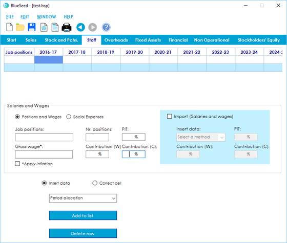
Just like in previous
tabs, first thing you see is a blank table (with the exception of the headers on
every column). Here you will see displayed every data you will be introducing afterwards.
In the case you could not see all the columns or rows
of this table, you can click on it and move through the cells with the arrow
buttons in your keyboard.
In fact there will be
two different tables, one for the data when you are working in “Positions and
Wages” option, and other for the information in “Social Expenses” one.
Anyway, the
information you will see in both tables will appear in following order: job
positions or social expenses denomination (in the first column), wage and
salaries total amounts for any job position or total amount for any expense by
period of time (next columns with the periods names in the header), finally, only
for “Positions and Wages” option, Personal Income Tax (PIT) rate, worker
Contribution (W) rate, company Contribution (C) rate, would be displayed for
every job position, if applicable, in the last three columns of related table,
which cannot be viewed in upper image.
To select the kind of
data you are working with, positions and wages or social expenses, you first
have to click on the consistent radio button, and follow as described in next
paragraphs.
There are two ways to
insert data in the tables: manually one by one or importing values from an
Excel worksheet.
In the first case you
should fill the different dialog boxes. When you are inserting positions and
wages figures you find a first textbox where you have to put the name of the
job positions in, beside there is another text box where you have to write the
number of positions for each job in the firm, and under you have another
textbox to introduce gross wage for that position. There are three more
textboxes where you can put in, whenever is necessary, Personal Income Tax
(PIT), worker Contribution (W), company Contribution (C) rates. Finally, you allocate
the period of time to which the data is related in the dropdown box just over
the “Add to list” button.
Otherwise, if you are
introducing social expenses information, you just have to write the name of the
expense in the first textbox and the expense total amount for that period in
the one below. Then again, you allocate the period of time to which the data is
related in the dropdown box just over the “Add to list” button.
If you want wages or
social expenses to be affected by CPI (the value you have introduced in the
first form), we tick on the checkbox labeled “Apply inflation”. The way in
which the program take into account the inflation rate is to apply a
coefficient to the gross wage you have written in corresponding textbox (which
should be a reference from the previous period to the first one in the project).
That coefficient is the result of multiply all the CPI rates (the ones shown in
the table in the firs tab) from the first period of time to the period you have
currently selected.
Now that you have all
the data you want to introduce in the table and the period of time where you
want to do it, you can insert that values by clicking on “Add to list” button.
To correct any of the
figures you have already introduced in the table, you count with two options: you
can delete a complete row (or product) just by selecting it and clicking on “Delete
row” button, or you can correct individual values cell by cell.
To change values in
only one cell you first have to select the radio button labeled as “Correct
cell”, then you have to select the cell by clicking on it and press “Correct”
button. A new window will appear where you have to introduce a new value, click
“OK” and the cell will show amended figure.
Import
You can only use this option when working in “Positions and Wages” selection.
As explained before, the application allows data import from an Excel worksheet,
as an alternative to inserting numbers one by one as described in the manual
method above.
To start this option you have to check “Import” box,
write Personal Income Tax (PIT),
worker Contribution (W), company Contribution (C) rates if applicable
within the textboxes enabled, and then select one of the two methods the
dropdown box offers to the users:
1)
Data Import
First option is plain data import, once you have
chosen the Excel file where you have the information you want to import, in the
dialog window appearing after clicking on the corresponding dropdown box item,
you will see a similar form to the previous ones (CPI and Interest rate, Sales
import methods), and also process to follow is quite similar.
First of all, you should put the cells range containing
the data to import in the textbox labeled that way, but here there is a
difference this time in the way the values has to be positioned. They should be
organized in a similar way the application ask for values when using the manual
method, so there are two key factors to have in mind before organize the
information in the Excel worksheet:
I. First column of the
range should contain the name of the job positions (with as many rows or fields
as you need).
II. After this first
column, they should follow pairs of columns for each same period of time (gross
wages and number of posts for each position, and should be as many pairs of
columns as periods of time in the project), with the same number of rows than
the first one.
Next step is to write the name of the Excel worksheet
in the next textbox under the previous one.
Then you click on “Import” and wait until the blank table
is filled with the names and numbers in the Excel file (this process could take
long if the selected range is too big).
If everything has worked out correctly and the values
in the table are the ones you wanted, you can click on “OK”, otherwise you can
repeat the process checking the range and name of the Excel worksheet.
2)
Time Series
The second item listed in the “Insert data” dropdown
box within import section is “Time Series”. blueSeed Plan provides another calculation method to
estimate total wages figures for each period of time (for only one field or job
position each time). It do it according to historic data trends (data provided
by the user), adding every new obtained value to the original series and using
increased set of values for the calculation of the next period of time rate.
Once you have the Excel file, where you keep the data
series, selected (cells values can only be numbers, this option do not accept
text) you will see a similar form to the previous one. Here you will first have
to put the cells range in the upper textbox, it can have several rows and columns,
if it has more than one row, the application takes values from left to right
and top to bottom.
Then you write the name of the Excel sheet in the
bottom textbox.
It is important to note that, firstly, the program
asks only for historic wages and salaries figures (not individual wage nor numbers
of position to make a multiplication), and there is no need neither to
introduce names of the posts in the first column as before (application will
assign a default name).
Next thing you click on “Import and calculate” and
wait until the blank table is filled with the numbers calculated by the
application (this process could take long if the selected range is too big).
When the program has finished calculation of the total
amount of payroll for each period of time, it announce the user he could now
introduce total number of job positions for each period, another table appears
where we can write, manually this time, the total quantity numbers for each
period (this table can be left totally blank as it has not impact in sales now
that the first table is completed).
If everything has worked out correctly and the figures
in both tables seem to be right, you can click on “OK”, otherwise you can
repeat the process checking the range and name of the Excel worksheet.
12. Overheads
“Overheads” tab
displays as follows:
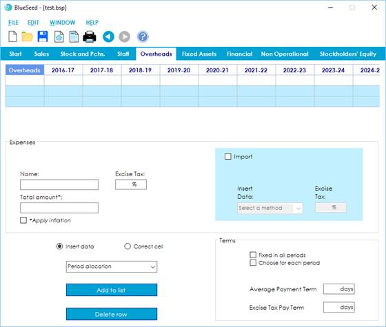
Like it happened in
previous sections, first thing you see is a blank table (with the exception of
the headers on every column) where you will see displayed every data you will
be introducing afterwards: name of the expenses (in the first column), expenses
amounts by period of time (next columns with the periods names in the header), average
and excise tax pay terms by period of time (which will be shown in the last two
blue rows) and, finally, excise tax rate by expense (in the last column of the
table, which cannot be viewed in upper image).
In the case you could not see all the columns or rows
of this table, you can click on it and move through the cells with the arrow
buttons in your keyboard.
There are two ways to
insert data in the table: manually one by one or importing values from an Excel
worksheet.
In the first case you
should fill the different dialog boxes: expense name in the first textbox, excise
tax rate and expenditure total amount in the second textbox. Then you should allocate
a period of time in the dropdown box just over the “Add to list” button.
If you want expenses to
be affected by CPI (the value you have introduced in the first form), we tick
on the checkbox labeled “Apply inflation”. The way in which the program take
into account the inflation rate is to apply a coefficient to the total amount
value you have written in corresponding textbox (which should be a reference
from the previous period to the first one in the project). That coefficient is
the result of multiply all the CPI rates (the ones shown in the table in the
firs tab) from the first period of time to the period you have currently
selected.
Now that you have all
the data you want to introduce in the table and the period of time where you
want to do it, you can insert that values by clicking on “Add to list” button.
Average and Excise Tax
pay terms are added separately selecting one of the two options in the “Terms”
section, fixed for all the project, with means they would be the same terms in
all the periods of time, or you can select to put different terms period by
period (in this case you will see that the dropdown box used to allocate
periods is enabled).
To correct any of the
figures you have already introduced in the table, you count with two options: you
can delete a complete row (or product) just by selecting it and clicking on “Delete
row” button, or you can correct individual values cell by cell.
To change values in
only one cell you first have to select the radio button labeled as “Correct
cell”, then you have to select the cell by clicking on it and press “Correct”
button. A new window will appear where you have to introduce a new value, click
“OK” and the cell will show amended figure.
Import
As explained before, the application allows data
import from an Excel worksheet, as an alternative to inserting numbers one by
one as described in the manual method above.
To start this option you have to check “Import” box,
write excise tax rate if applicable within the textbox enabled, and then select
one of the two methods the dropdown box offers to the users:
1)
Data Import
You have to choose the Excel file where you have the
information you want to import, in the dialog window appearing after clicking
on the corresponding dropdown box item, you will see then a similar form to the
previous ones (CPI and Interest rate, Sales, Purchasing import methods), and
also process to follow is quite similar.
First of all, you should put the cells range
containing the data to import in the textbox labeled that way, but here there
is a difference this time in the way the values has to be positioned. They
should be organized in a similar way the application ask for values when using
the manual method, so there are two key factors to have in mind before organize
the information in the Excel worksheet:
I. First column of the
range should contain the name of each expense (with as many rows or fields as
you need).
II. After this first
column, they should follow columns with total amount spent in that overhead for
each period of time (not pairs of columns as in other sections of the program),
with the same number of rows than the first one.
Next step is to write the name of the Excel worksheet
in the next textbox under the previous one.
Then you click on “Import” and wait until the blank table
is filled with the names and numbers in the Excel file (this process could take
long if the selected range is too big).
If everything has worked out correctly and the values
in the table are the ones you wanted, you can click on “OK”, otherwise you can
repeat the process checking the range and name of the Excel worksheet.
2) Time Series
The second item listed in the “Insert data” dropdown
box within import section is “Time Series”. blueSeed Plan provides another calculation method to
estimate total overheads for each period of time (for only one expense each
time). It do it according to historic data trends (data provided by the user),
adding every new obtained value to the original series and using increased set
of values for the calculation of the next period of time rate.
Once you have the Excel file, where you keep the data
series, selected (cells values can only be numbers, this option do not accept
text) you will see a similar form to other sections ones. Here you will first
have to put the cells range in the upper textbox, it can have several rows and
columns, if it has more than one row, the application takes values from left to
right and top to bottom.
Then you write the name of the Excel sheet in the
bottom textbox.
It is important to note that, firstly, the program
asks only for historic overheads figures (not costs and numbers of services to
make a multiplication), and there is no need neither to introduce names of the expenses
in the first column as before (application will assign a default name).
Next thing you click on “Import and calculate” and await
until the blank table is filled with the numbers calculated by the application
(this process could take long if the selected range is too big).
If everything has worked out correctly and the figures
in the table seem to be right, you can click on “OK”, otherwise you can repeat
the process checking the range and name of the Excel worksheet.
13. Fixed Assets
Below you can see a
screenshot of “Fixed Assets” tab when it is selected by user:
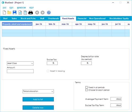
In this one, and some
of the following tabs, gathering information is a little bit different. Application
will not request for data in every period of time, it will just ask for opening
values or references and will automatically calculate the rest in each period, taking
into account all parameters introduced. Also, there is no possibility for data
import.
Again you have a
blank table (with the exception of the headers on every column) where you will
see displayed every data you will be introducing afterwards: name of assets (in
the first column), their end of period value (next columns with the periods
names in the header), average and excise tax pay terms by period of time (which
will be shown in the last two blue rows), excise tax rate by expense (in the
next-to-last column, not seen in the image above) and, finally, depreciation
rate (in the last column of the table, not seen in the image above).
In the case you could not see all the columns or rows
of this table, you can click on it and move through the cells with the arrow
buttons in your keyboard.
So, to load the
information in the table you first have to choose an asset in the list of the
dropdown box called “Asset Class”. Items in the list are: (first intangible
assets) I+D Expenses, Administrative License, Goodwill, ICT Apps; (then
property, plant and equipment) Buildings, Equipment, Furniture, Technical
Facilities, Vehicles and Land.
In the textbox below
you should write asset purchase price or market value (without excise tax). Then
you can write an excise tax rate in the textbox labeled accordingly, if that is
applicable, and finally put the consistent depreciation rate in the last textbox.
If you have used a
leasing contract to support the acquisition of any particular asset, so it is
linked to that financial debt, you should check on “Asset in leasing” box. It
is important you do it because, otherwise, program would already have a
financial debt (leasing) reflected in its reports, and would have another (fixed
asset supplier outstanding debt), at the end of period.
To set the date of
the asset acquisition you, as usual, have to select a period of time in the
dropdown box called “Period allocation” and click on “Add to list” button. After
that the program will calculate asset end of period value, deducting
accumulated depreciation.
Average and Excise Tax
pay terms are added separately selecting one of the two options in the “Terms”
section, fixed for all the project, with means they would be the same terms in
all the periods of time, or you can select to put different terms period by
period (in this case you will see that the dropdown box used to allocate
periods is enabled).
To correct any of the
figures you have already introduced in the table, you only count with one
option this time: you should delete a complete row (or asset) just by selecting
it and clicking on “Delete row” button.
14. Financial
Hereunder you can
find a screenshot of this tab:
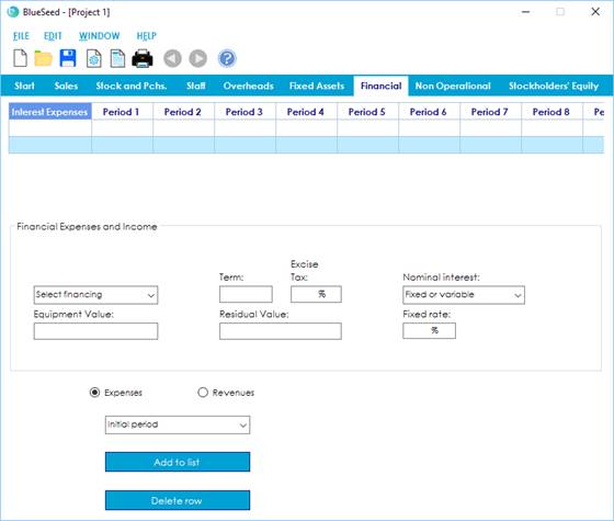
Just as in the
previous tab, you have to provide the starting values and parameters of the
selected financial asset or liability, and the application calculates the
resulting data for the rest of the periods.
But first choice to
make is to select between financial expenses or revenues (each kind of data
will be recorded in a different table). For that, we check on the matching
radio button “Expenses” or “Revenues”.
In any choice you
have a blank table (with the exception of the headers on every column) where
you will see displayed every data you will be introducing afterwards: name of
assets or debts (in the first column) and accrued interest receivable or
payable by periods (next columns with the periods of time names in the header).
In the case you could not see all the columns or rows
of those tables, you can click on it and move through the cells with the arrow
buttons in your keyboard.
So to calculate and
display the figures in the tables, either you have selected expenses or
Revenues, you have to choose one item in the first dropdown box in the section.
For “Select financing” box the possibilities are: Leasing (post), Leasing
(pre), Renting, Loan and Credit Account; and for “Type of investment” one the
list is: Fixed term deposit and Loan.
In the textbox below
you can put the amount of the debt (or equipment cost or market value) or the credit.
Then you can set the length of the financial operation itself by write a number
in the “Term” labeled box.
In the cases of leasing
or renting debt operations, there are some other parameters you can make use
of: residual value, other expenses inherent to that operation (for renting), and
excise tax rate. As for Loans you can add a grace period.
But one of the most
important factor in every financial contract is interest. Here, the application
gives you two options:
We can select a fixed
interest for that particular operation, so you will have to pick that item in “Nominal
interest” dropdown box and write an interest rate in the textbox below.
On the other hand, if
you want a variable interest rate for every period, after picking that
selection in the dropdown box, you would have to put a rate differential (it
can be 0) that will sum up to the benchmark rate of our project (which is the
one introduced in the first form when opening a new project, and that is
displayed in “Start” tab).
Lastly, as usual, we
choose opening period for the contract, either debt or asset, and click on “Add
to list”. The program will calculate and display in the table the amount of interests
for that kind of operation in any period to the end of contract term (or project
life if this one is shorter).
To correct any of the
figures you have already introduced in the table, you only count with one
option this time: you should delete a complete row just by selecting it and
clicking on “Delete row” button.
15. Non Operational
Following tab is for
Non Operational expenses or revenues and it has this sight:
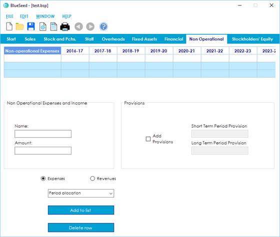
In this section you
have to introduce data period by period, in part is like first stages of the
application (but it cannot import values).
What you first see, other
than the usual blank table, is that there are two parts and only one is operational
at the same time, and by default is the first one (the one in the left) which
is enabled. To revert that situation you just have to click on “Add provisions”
box what will deactivate first group and activate “Provisions” one.
Left part of the
section “Non Operational Expenses and Income” is used basically for that, to introduce
non operational values in one of the tables (expenses or revenues), so first
choice to make is to select between them (each kind of data will be recorded in
a different table). For that, we check on the matching radio button “Expenses”
or “Revenues”. Then you have a textbox to write the name of the expense or
revenue and another one to put the amount for a given period of time in.
Finally you select the period in “Period allocation” dropdown box and click on
“Add to list”.
Tables are organized
as in previous tabs, in the first column the name of the expense or revenue
will be shown, and its amounts by period in the following columns. The last two
blue rows are reserved for provisions.
In the case you could not see all the columns or rows
of those tables, you can click on it and move through the cells with the arrow
buttons in your keyboard.
The group “Provisions”
in the right part allow you to manage short and long term provisions, and as
explained before, it has to be activated before start working with it.
After checking on
provisions box, first thing you note is that labels in radio buttons below change
for “Provisions of period” and “Provisions Surplus” accordingly. This make no
difference operationally (as they continue to distinguish between the same
tables you were using before), just announce what kind of provision movement you
are going to carry out, a period provision (equals an expense in income
statement) or a provision surplus (equals a revenue in income statement).
Hence, to copy the
values in the table you have to select one radio button and fill the textboxes
inside the group: figures for short term in the upper one and long term values
in the lower one.
Finally you follow as
usual, you should allocate a period of time in the dropdown box just over the
“Add to list” button and click on the later.
To correct any of the
figures you have already introduced in the table, you only count with one
option this time: you should delete a complete row just by selecting it and
clicking on “Delete row” button.
16. Stockholders’ Equity
Last tab, to complete
the introduction of all information needed by the application, has this view:
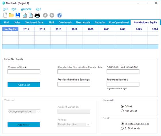
As you can see in the
previous image, there are several groups where you must put the values you want
to record in the project.
In the first one
“Initial Net Equity”, you see different textboxes you can fill: Common Stock, Shareholders
Contribution Receivable, Additional Paid-In Capital, Previous Retained Earnings
and Recorded Losses.
In all five boxes you
should write opening values for each Net Equity field (those quantities should
be the same the ones you have in starting balance sheet of the new project).
Common Stock value is
a must you should fill, to have intelligible reports and to calculate some of
the financial ratios this program offers (as IRR). The applications offers the
opportunity to add capital increases after first period, as you will see later.
Rest of the textboxes
are optional to fill. Shareholders Contribution Receivable and Additional
Paid-In Capital values can be modified after having set opening values, as you
will see later. Movements in this variables would then affect to cash flow
report or to financial rates too.
Previous Retained
Earnings and Recorded Losses can be left blank, in the case your Project is related
to a new undertaking, or use the figure in balance sheet in the case of ongoing
companies.
Once you have written
all the initial values you want to record, just click on the upper “Add to list”
button to display them in the table. This action also enable the second group
of controls “Variation”, and disable the first one (there is an option to come
back to this group as you will see later).
In the case you could not see all the columns or rows
of this table, you can click on it and move through the cells with the arrow
buttons in your keyboard.
Now, in this group
you first can appreciate a dropdown box which has four options to choose:
Common Stock Increase, Additional Paid-In Capital, Shareholder Contribution Receivable
Deposit and Change Origin Values.
So, to make changes
in the displayed numbers, we have to select one of the first three items, last
one just disable this section and returns you to the first one. Then, write the
variation amount in the next textbox and, finally, allocate the period of time
when this adjustment would happen. Last of all you just have to click on “Add
to list” in this group, and the program will recalculate the balance of every
field on the table taking into account the new adjustments, and new values will
display in the table.
Last parts of the tab
are two sections where you can take decisions about tax credit and retained
earnings.
Within “Tax credit”
section, you have two options to choose: Offset or Not Offset negative tax
bases (coming from previous periods). If you choose to offset tax bases, any period
you have an income tax positive quota it will be diminish in the corresponding
amount. In the case you choose not to offset tax bases, any negative new tax
base will be added to Recorded Losses in balance sheet.
In conclusion, within
“Profit” section, you can choose destination of earnings surpluses in every
period of time, and you have two options: To Retained Earnings and To Dividends.
If you choose first choice, every net income would add to Retained Earnings in
the balance sheet (increasing net equity total amount). On the other hand, if
you decide to distribute dividends,
the program considers there is cash outflow (and there is no increasing in net
equity).
17. Reports View / Print (  /
/  )
)
Most important
utility of blueSeed Plan is the production of several kind of reports, graphics
and financial ratios using all the information you have introduced in every
stage in the application.
Reports can be viewed
in the screen, for what you have to click on button ![]() in the toolstrip, or can be sent directly to printer just by
clicking on button
in the toolstrip, or can be sent directly to printer just by
clicking on button ![]() (there is the possibility to export to an
Excel file as you will see later).
(there is the possibility to export to an
Excel file as you will see later).
After clicking on any
of the described buttons, a new dialog window will appear (as it is shown in
the following image), where you can select which reports, budgets, graphics you
want, and in which units they will be displayed.
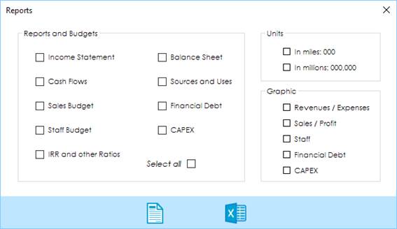
Once we have chosen
the reports we want to see or print by checking on the matching box, you have
to click on one of the two buttons this window shows: view at the screen ![]() or print
or print
![]() it (depending on the choice you have done in
prior step), and export to Excel file
it (depending on the choice you have done in
prior step), and export to Excel file ![]() .
.
18. Full Screen
Usually, tables
displaying data in every tab of the main form are not big enough to see all their
rows or columns, therefore not having all information at only one view. To somewhat
sort this out, you can double-click on any table and it will be rendered in
full screen.
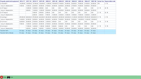
In some cases: Fixed
Assets, Financial and Stockholders’ Equity, you will see more information in this
mode than when not using full screen. This data, though used by the application
to make up the reports, is made not visible by the program to try to summarize the
most significant values in tab table smaller area.
For instance, if you
double-click in “Fixed Assets” tab table, you will see something like this
image hereunder:
And a clearer detail
of it would be:
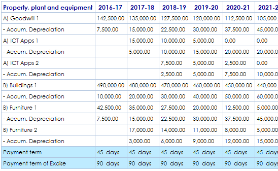
Here you can see
that, below the row of every fixed asset, there is another with the related
accumulated depreciation.